Written by Hillis Burns, Shannon Timoney, Hall Pritchard (students in Math 383D Knot Theory Spring 2023).
We created the T(2, 8) torus link (or 821 link) using Cinema 4D. The equations for this two component link are x = Cos[t]*(3+Cos[4t]), y = Sin[t]*(3+Cos[4t]), and z = Sin[4t]. The second component is created by the equations x = Cos[t]*(3+Cos[4t+Pi]), y = Sin[t]*(3+Cos[4t+Pi]), and z = Sin[4t+Pi].
We also created the T(3, 3) torus link (or 632 link). With the 632 link, each of the three components goes around the longitude once and goes around the meridian once. The equations for this knot are x1 = Cos[t]*(3+Cos[t]), y1 = Sin[t]*(3+Cos[t]), z1 = Sin[t], x2 = Cos[t]*(3+Cos[t+2*Pi/3]), y2 = Sin[t]*(3+Cos[t+2*Pi/3]), z2 = Sin[t+2*Pi/3], and x3 = Cos[t]*(3+Cos[t+4*Pi/3]), y3 = Sin[t]*(3+Cos[t+4*Pi/3]), z3 = Sin[t+4*Pi/3].

The T(3,3) torus link shown lying on the torus.
After creating the T(3, 3) or 632 link, we wanted to build a model that helps demonstrate what the torus link actually is. We did this by first opening back up the T(3, 6) or 632 in Cinema 4D. Then we created a torus surface and rotated it 90° so that the torus link sat in the right position on the torus surface. Then we changed the radius of both the meridian and the longitude so that the 3d model was in a presentable format. Our final model which is shown above gives a good physical representation of how a torus link is constructed.
We also created the T(3, 6) torus link (or 633 link). With the 633 link, each of the three components goes once around the longitude and goes three times around the meridian. The equations for this knot are x1 = Cos[t]*(3+Cos[2t]), y1 = Sin[1t]*(3+Cos[2t]), z1 = Sin[2t], x2 = Cos[t]*(3+Cos[2t+2*Pi/3]), y2 = Sin[t]*(3+Cos[2t+Pi]), z2 = Sin[2t+2*Pi/3], and x3 = Cos[t]*(3+Cos[2t+4*Pi/3]), y3 = Sin[t]*(3+Cos[2t+4*Pi/3]), z3 = Sin[2t+4*Pi/3].
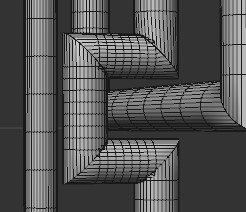
While using the Cinema 4D software, the biggest problem we had was fixing the join at the end of two strands. In Cinema 4D, the join will sometimes not look correct. In order to fix this, we will first decrease the period of the parametric equations in order to make the join fully noticeable. We decreased it from 2π (~6.28) to 6.275.

Too many points are highlighted near the ends of the torus link.
We then try to highlight all the points at the end of the knot, in order to use the “stitch and sew” function. We came across problems when we accidentally highlighted other points not at the end. This is shown in the figure to the right. This would happen more often when we increased the sample size to a number that was higher than necessary (>300). This is the case in the image below. By decreasing the sample size, it made it easier to highlight just the end points of the knot, as shown below. At this point we were able to successfully use the “stitch and sew” function.

This image shows that just the end points of the two ends of the torus link are highlighted. This allowed us to successfully use the Stitch and Sew function to join the ends together.