 The Lorenz attractor is a set of chaotic solutions of the Lorenz system which, when plotted, resemble a butterfly or figure eight. The Lorenz system is a system of ordinary differential equations first studied by Edward Lorenz in the 1960’s. It is notable for having chaotic solutions for certain parameter values and initial conditions.
In Winter 2015, my colleague Professor Greg Dresden used the Lorenz attractor as an example in his course on Partial Differential Equations. At that time, I worked with Dave Pfaff in the IQ center at W&L to find a way to 3D print a physical model of the solution curves. Dave also created model of the solution curves that could be viewed with 3D glasses in our stereo 3D lab. To create the models we followed three steps:
Step 1: Create points along the solution path (the Lorenz curve) using Mathematica. Here is the Mathematica code Greg developed for this purpose.
(* Here are the differential equations *)
leqns = { x'[t] & == -3 (x[t] – y[t]),
y'[t] & == -x[t] z[t] + 28 x[t] – y[t],
z'[t] & == x[t] y[t] – z[t] };
(* Here, I define two paths, p1 and p2, which start at slightly-different initial values. *)
p1 = NDSolveValue[{leqns, x[0] == z[0] == 0, y[0] == 1}, Function[Evaluate[{x[\#], y[\#], z[\#]}]], {t, 0, 30}];
p2 = NDSolveValue[{leqns, x[0] == z[0] == 0.03, y[0] == 1}, Function[Evaluate[{x[\#], y[\#], z[\#]}]], {t, 0, 30}];
(* Let’s look at a plot of these two paths, to verify that they seem correct *)
pic1 = ParametricPlot3D[p1[t], {t, 0, 30}, AxesLabel -> {x, y, z}, PlotStyle -> {Red, Opacity [0.5]}];
pic2 = ParametricPlot3D[p2[t], {t, 0, 30}, AxesLabel -> {x, y, z},
PlotStyle -> {Black, Opacity [0.5]}];
(* Finally, we export them as two separate files *)
tableout1 = Table[p1[t], {t, 0, 30, 0.01}];
tableout2 = Table[p2[t], {t, 0, 30, 0.01}];
Export[“TableOut1.xls”, tableout1]
Export[“TableOut2.xls”, tableout2]
Step 2: Use Excel to tweak the data into a form we can use.
- Open the files in Excel.
- Insert a column before the three columns of numbers, this is column A. Make the first row 1, and the second row 2 in column A.
- Highlight these two entries in column A, then drag the box down to row 3001. The numbers in column A will automatically fill in the correct numbers.
- Highlight all of the numbers in all four columns. Click on Save As, then save the file as a Tab Delimited Text (.txt) file.
Step 3: Create the thickened Lorenz curve in Cinema 4D.
- Open Cinema 4D
- Construct the spline with the Lorenz data.
- Left click and hold on the Spline button on the top row, then select the Linear (spline) button. Click once on the view-port to add one point.
- Go to the Object Manager. On the right side, click on the Structure button. You’ll see the Point 0, with X, Y and Z coordinates.
- Click on the File button above the Object Manager. Click on Import ASCII Data… Open the .txt file created above.
-
 Click on the 0th point (the one you added initially) and Delete it. The remaining points are from the Lorenz data (see figure.)
 - Click on the Objects button on the right side of the Object Manager.
- Thicken the spline for 3D printing.
- Left click and hold on the Subdivision Surface button on the top menu, then select the Sweep button.
- Left click and hold on the Spline button on the top row, then select the Circle button. Under the Attribute Manager, make the radius of the circle 3mm (0.3cm).
-
 In the Object Manager, move the Circle and the Spline under the Sweep. The Circle should be above the Spline (see figure). The thickened spline is now complete, and the Lorenz curve can now be exported (as a .stl file) and then 3D-printed.


A thickened Lorenz curve in Cinema 4D is shown below on the left. Two curves can be added to the same plot in Cinema 4D and given different colors. Dave Pfaff printed two such curves using the Project 260 3D printer at WLU. (This printer uses a gypsum-like powder hardened via a laser then finished with superglue.) The Project 3D printer can print in color (using inkjet cartridges). Dave also designed a stand for the curves. This gives the beautiful model shown below on the right. Cinema 4D also allows the user to animate the curves. Dave created such an animation, which nicely shows the chaotic nature of the Lorenz attractor. The initial points of the two curves were very close, but in the long term, the curves diverge.


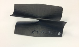
 I also had to reverse the normals on half of the object to make sure they were all aligned with the other half before I extruded the surface. I optimized the polygons to be sure the edges joined up into one object. I then extruded the surface to create my hyperboloid of two sheets. I copied this and put equations through one of them. I also made sure to Boole the edges of the hyperboloid to make them flat for printing.
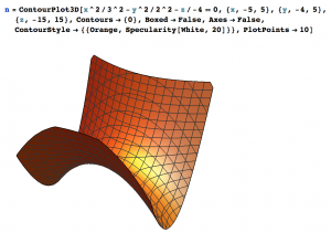 Once I had done this I did the same thing with the optimize tool in Cinema 4D to see how big I could make the polygons before the surface started to lose accuracy. The first time I went through all these steps the hyperbolic paraboloid I had chosen just didn’t work correctly. So, I went back to the beginning and created a new Mathematica file of a hyperbolic paraboloid, and spent some time deciding where to cut it off to create edges that were as straight as possible.


 Then I optimized the object by 0.02cm. With the first cone I made I reversed the normals so they were facing outwards from the cone surface. When I extruded the surface by 0.25cm this automatically gave center of the object more thickness. Unfortunately I realized that while it gave the center thickness, it also offset the lines of the cone so they didn’t match up, which is not what we wanted. In order to fix this problem I did the same thing but did not reverse the normals (so they were facing the inside) and extruded the surface to give the cone thickness.

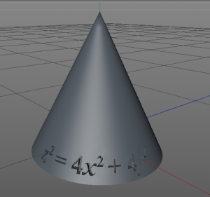 In order to do this I used the same formula spline except this time from only \(t=-2\) to \(t=0\) and copied and rotated it to create the second half. On one half I put the equation for the cone \(\frac{z^2}{4}=x^2+y^2\) and immediately ran into trouble. I had used too many subdivisions (72) and the object was not accepting the Boole with the equation. After creating many different cones with different subdivisions I found that 60 worked. Once this problem was solved I added the equations to one of the halves of my cone and printed it. When I added the equation I put it all the way through the surface and not just imprinted on it since the object had very little thickness to it.


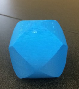
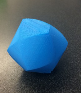
 The first print I did of the ellipsoid I cancelled the print early on so that I could inspect the sides. The surface looked a bit melty, where the filament had shrunk. We decided this was fine and to try to print it again.
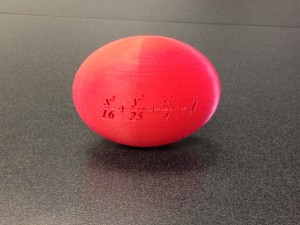 This time when I printed it I decided to put the equations on the top of the ellipse and use a raft. It printed perfectly.
 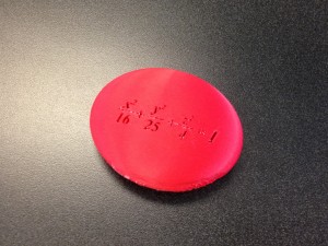 After my success with my second ellipsoid I decided to try to print my first ellipsoid again and this time with a raft. The object never fell over and printed perfectly. These ellipsoids can be found on Thingiverse


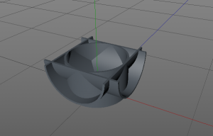 For the three cylinders I created them from scratch in Cinema 4D using the ‘Tube’ object. Creating the three cylinders was very straightforward. After my fail from the two cylinder object I also wanted to create the three intersecting cylinders cut in half, so the inside was visible. This proved to be a little more complicated. I used a ‘Cube’ and ‘Boole’ with each tube in order to get half cylinders. Then I was able to merge them together using a very similar process to putting equations on solids in Cinema 4D.