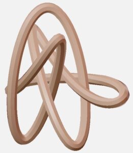
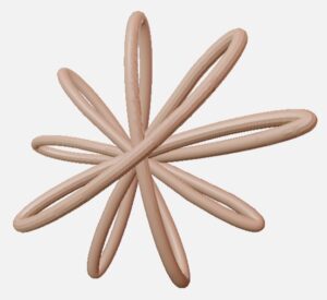
Written by Keally Rohrbacher and Sawyer Dunn-Matrullo (students in Math 383D Knot Theory Spring 2023).
Our plan was to create models of knots with petal projections. This is a particular type of diagram of knots that has only one crossing, and a certain odd number of arcs which cross each other there. For example, Figure 1 shows the petal projection of the Trefoil Knot (image from Wikipedia). The numbers written on the arcs in Figure 1 are important, as the order in which the knot crosses through itself is what distinguishes different petal projections of knots from each other.
We wanted to produce 3D models of the 41, 52, and 61 knots, all of which have petal projections (shown in the figures below).
Since it is not important what the actual picture of the petal projection is, just that it crosses through the center in a particular order, we had some choice as to how we were doing to construct these knots. We decided that it would be interesting to construct these as parameterized functions. We knew that we could make the x and y-components of this function fairly easily using a rose curve, a type of polar function which produces a cool rose that looks just like the petal projection in 2D. So, we knew that all we had to do was come up with a function for the z-axis which would parametrize the rose curve to go around and hit the center at certain heights to produce the petal we wanted. We knew which order the strand should go through the crossing in for each knot from the paper “Knot Projections with a Single Multi-Cossing” by Colin Adams and his coauthors.
We considered a couple ideas for finding a function that would hit these particular heights, but ultimately decided to try to find a polynomial function.
We did this by creating points with the heights we needed to hit at even intervals and plugged these points into an online calculator which uses Lagrangian interpolation to produce a polynomial which hit all of these points. Once we defined this as the z-component for our function, and used the rose curve for the x- and y-components, we plugged our curve into a 3D graphing calculator called GeoGebra. The side views, in figures 2, 4 and 6 (above and below), depict these heights being hit in proper order in accordance with the Adams’ paper. The top views in figures 3, 5 and 7 show the petal projection shape of the rose curve projected to the xy-plane.
We ran into a couple issues during this project. The most annoying of which was trying to define our curve as a parametrized function in Cinema 4D.
Because we had to hit so many points, the function on the z-axis ended up being a degree 11 polynomial for both knots. And while we were able to produce this on GeoGebra, a powerful calculator, we could not make a satisfactory spline of our function in Cinema 4D. We spent a long time trying to fix this problem by manipulating points on the software. We were exasperated to find that we could simply download an .stl file directly from GeoGebra, where we already had constructed the knot, circumventing our entire issue. (Note that 3D printers use .stl files as their start point.) This made its own set of issues, however, as the shapes from GeoGebra were not smooth. But, for our final print of the knots, we also graphed the curves on Mathematica like we did in GeoGebra, again avoiding the issue of plotting a curve in Cinema 4D and Mathematica gave us models with much smoother curves.
The most challenging part of coming up with our functions though was creating and working with high order polynomials, but this mostly just involved us typing out long equations many times. We found that WolframAlpha easily came up with the required higher order polynomials for the 61 knot (which ended up being a degree 14 polynomial).


