Written by Chadrack Bantange and JCW (students in Math 383D Knot Theory Spring 2023).
Background:
What is a minimal cubic lattice knot?

The cubic lattice.
Let’s start with: what is the cubic lattice? The cubic lattice is all the points (a, b, c) in R3 such that a, b, c are integers. That is, the cubic lattice is composed of all the points in three dimensions that have integer entries. The image to the right is a depiction of the cubic lattice (from Wolfram MathWorld).
Next, what would it mean for a knot to be in the cubic lattice? Cubic lattice knots are knots whose vertices lie in the cubic lattice. That is, the vertices of the knot can be represented by (a, b, c) where a, b, c are integers.
Another way to think about cubic lattice knots would be to imagine you start your knot on the point (0, 0, 0). To take a step tracing the knot one must take one of the steps as depicted below. Observe that on this first step from the origin one has six options. One could go: left, right, up, down, forward, or back. Consider the diagram below which presents all six of the options. The step which traces the knot is itself not a part of the cubic lattice. If we move up from the origin to point (0, 0, 1) all the points between these vertices makeup the knot, but are not part of the cubic lattice per se.

Figure showing the 6 points in the cubic lattice one unit from the origin.
In each of the subsequent steps you have similar options. Because you are walking within the cubic lattice, on each step you can only ever add +1 or -1 to just one of your x, y, or z coordinates to get your next vertex. Note: since we are drawing a knot, you will have one less option than when starting at the origin, because you do not want to walk back on the knot you have already drawn. If you go up from (0, 0, 0) to (0, 0, 1), then you could not go back down to (0, 0, 0) when tracing your knot.
Lastly, what is a minimal cubic lattice knot? Each knot has multiple equivalent representations and diagrams that can be reached via planar isotopies and Reidemeister moves. This means there are many versions of each kind of knot in the cubic lattice.
Consider the trefoil. One could trace a trefoil knot in the cubic lattice that globally looked somewhat smooth and like a common depiction, as below on the left. This, however, is not particularly mathematically interesting or remarkable. Rather, to ask the more interesting question we ask: what is the minimal cubic lattice knot? That is, for each of the knot equivalence classes what is the shortest walk we could take in the cubic lattice to trace out a knot in the equivalence class? On the right, observe the minimal cubic lattice knot for the trefoil. In the case of the trefoil (31), the minimal walk in the cubic lattice is 24 steps. (Left image from the Rolfsen Knot Table Mosaic.)
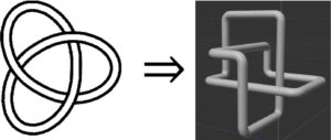
Figure showing the standard image of the trefoil knot (left), and the image of the minimal length trefoil in the cubic lattice (right).
Construction
To build the cubic lattice knots, we used Cinema 4D. As part of this process, we referred to Andrew Rechnitzer’s website on plotting minimal cubic lattices). For all the cubic lattices, we noticed that when importing the data from Notepad into Cinema 4D, one line of the coordinates was missing, making the object look incomplete. This was a challenge we experienced in constructing our knots. Correcting this issue involved manually attaching numbers to each line of the coordinates while also inserting a row of zeros in the first line of the dataset. As we went on building more knots, we noticed that this process was time-consuming. Alternatively, we used Microsoft Excel to copy our coordinates from Notepad, pasted into Excel using the “paste special” option, and we were able to use Excel to automatically attach numbers to the individual coordinates. We then pasted these coordinates back into Notepad and saved it as a “txt” format.
Once the data was imported into Cinema 4D, we went to “view” in the left menu, selected “Frame Geometry” to get a better geometric view of the knot. The spline automatically connected all the points except the last to the first. Before connecting them, we first made sure that under Object manager, we have “Rectangle—Spline” selected; under “Attributes—Object—Type” , choose “bezier or linear” depending on how smooth we want the corners of the knot to look like. For some of the knots, “bezier” was the best smoother of the corners, while for others, “linear” was best. To connect the vertices, we selected “spline pen” and were able to click on the two, unconnected points to add the last edge to the spline.
At this point all we had was a spline made of 1-dimensional lines. In order to make the knot 3-dimensional for printing and visualization, we added “circle” and “sweep” to our Cinema 4D workspace. The circle would serve as the cross section for our knot and the sweep is what swept the circle cross section along the spline we created above. We then adjusted the radius of the knot, which in most cases was 0.25 cm. In order to smooth out the corners, we added a Chamfer to the knots and set its radius at 0.25 cm for the 3, 4, 5, and 6 crossing knots and 0.3 cm for the 7 crossing cubic knots. We then scaled the object to be hand sized. There were a lot of variations in this regard depending on the knot, especially since some of the minimal cubic lattice knots occupied the space of a cube, while others occupied the space of a rectangular prism. In general, however, the scale ranged from 4 to 8 cm in all the three axes (x,y,z). We saved both .stl and .c4d files, ready to be printed in the IQ center at WLU.
Here are some screenshots of our work. In both cases, the standard image of the knot came from the Rolfsen Knot Table Mosaic.

On the left, the standard view of 5_2 knot. On the right, the minimal cubic lattice knot of 5_2.

On the left the standard view of the knot 6_1. On the right the minimal cubic lattice knot of 6_1.


