 The Lorenz attractor is a set of chaotic solutions of the Lorenz system which, when plotted, resemble a butterfly or figure eight. The Lorenz system is a system of ordinary differential equations first studied by Edward Lorenz in the 1960’s. It is notable for having chaotic solutions for certain parameter values and initial conditions.
In Winter 2015, my colleague Professor Greg Dresden used the Lorenz attractor as an example in his course on Partial Differential Equations. At that time, I worked with Dave Pfaff in the IQ center at W&L to find a way to 3D print a physical model of the solution curves. Dave also created model of the solution curves that could be viewed with 3D glasses in our stereo 3D lab. To create the models we followed three steps:
Step 1: Create points along the solution path (the Lorenz curve) using Mathematica. Here is the Mathematica code Greg developed for this purpose.
(* Here are the differential equations *)
leqns = { x'[t] & == -3 (x[t] – y[t]),
y'[t] & == -x[t] z[t] + 28 x[t] – y[t],
z'[t] & == x[t] y[t] – z[t] };
(* Here, I define two paths, p1 and p2, which start at slightly-different initial values. *)
p1 = NDSolveValue[{leqns, x[0] == z[0] == 0, y[0] == 1}, Function[Evaluate[{x[\#], y[\#], z[\#]}]], {t, 0, 30}];
p2 = NDSolveValue[{leqns, x[0] == z[0] == 0.03, y[0] == 1}, Function[Evaluate[{x[\#], y[\#], z[\#]}]], {t, 0, 30}];
(* Let’s look at a plot of these two paths, to verify that they seem correct *)
pic1 = ParametricPlot3D[p1[t], {t, 0, 30}, AxesLabel -> {x, y, z}, PlotStyle -> {Red, Opacity [0.5]}];
pic2 = ParametricPlot3D[p2[t], {t, 0, 30}, AxesLabel -> {x, y, z},
PlotStyle -> {Black, Opacity [0.5]}];
(* Finally, we export them as two separate files *)
tableout1 = Table[p1[t], {t, 0, 30, 0.01}];
tableout2 = Table[p2[t], {t, 0, 30, 0.01}];
Export[“TableOut1.xls”, tableout1]
Export[“TableOut2.xls”, tableout2]
Step 2: Use Excel to tweak the data into a form we can use.
- Open the files in Excel.
- Insert a column before the three columns of numbers, this is column A. Make the first row 1, and the second row 2 in column A.
- Highlight these two entries in column A, then drag the box down to row 3001. The numbers in column A will automatically fill in the correct numbers.
- Highlight all of the numbers in all four columns. Click on Save As, then save the file as a Tab Delimited Text (.txt) file.
Step 3: Create the thickened Lorenz curve in Cinema 4D.
- Open Cinema 4D
- Construct the spline with the Lorenz data.
- Left click and hold on the Spline button on the top row, then select the Linear (spline) button. Click once on the view-port to add one point.
- Go to the Object Manager. On the right side, click on the Structure button. You’ll see the Point 0, with X, Y and Z coordinates.
- Click on the File button above the Object Manager. Click on Import ASCII Data… Open the .txt file created above.
-
 Click on the 0th point (the one you added initially) and Delete it. The remaining points are from the Lorenz data (see figure.)
 - Click on the Objects button on the right side of the Object Manager.
- Thicken the spline for 3D printing.
- Left click and hold on the Subdivision Surface button on the top menu, then select the Sweep button.
- Left click and hold on the Spline button on the top row, then select the Circle button. Under the Attribute Manager, make the radius of the circle 3mm (0.3cm).
-
 In the Object Manager, move the Circle and the Spline under the Sweep. The Circle should be above the Spline (see figure). The thickened spline is now complete, and the Lorenz curve can now be exported (as a .stl file) and then 3D-printed.


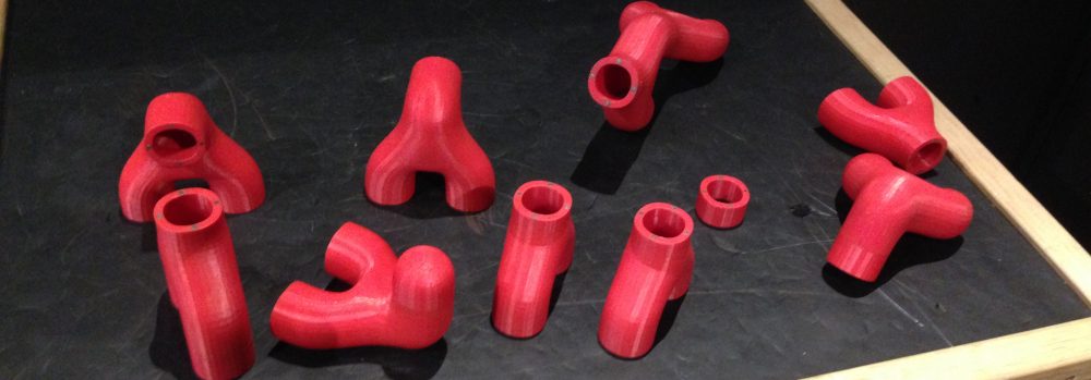
A thickened Lorenz curve in Cinema 4D is shown below on the left. Two curves can be added to the same plot in Cinema 4D and given different colors. Dave Pfaff printed two such curves using the Project 260 3D printer at WLU. (This printer uses a gypsum-like powder hardened via a laser then finished with superglue.) The Project 3D printer can print in color (using inkjet cartridges). Dave also designed a stand for the curves. This gives the beautiful model shown below on the right. Cinema 4D also allows the user to animate the curves. Dave created such an animation, which nicely shows the chaotic nature of the Lorenz attractor. The initial points of the two curves were very close, but in the long term, the curves diverge.


