A polygonal knot is a knot that is built from a finite number of straight line segments or edges. Two edges meet at a vertex of the knot. A polygonal knot can thus be described by listing the vertices v1, …, vn. The edges join each pair of vertices: e1 = v1v2, e2 = v2v3, …, en = vnv0. An equilateral stick knot is a polygonal knot where each of the edges has the same length.

A collection of 3D printed equilateral stick knots. Top row: 9:29 and 9_36. Bottom row: 8_13, 7_4 and 8_17.
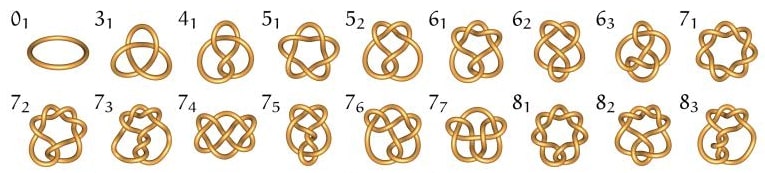
One of the many open problems in knot theory is to find the least number of edges or sticks needed to build a particular knot. This number is referred to the stick number s(K) of a knot K. The stick number of a few of the simplest knots is known. For example: s(unknot)=0, s(trefoil)=6, s(figure 8)=7. There are a number of results giving upper and lower bounds of the stick number in terms of the crossing number of a knot. These inequalities can be combined with physical constructions of a particular knot to prove a given stick number. In a similar fashion, the equilateral stick number can be found for a knot. This is the least number of equal length sticks needed to build a particular knot. It is an open question as to whether the equilateral and regular stick numbers are the same. In the not too distant past, Eric Rawdon and Rob Scharein (Knot Plot) produced a list of knots through 10 crossings for which they could not match the stick number and equilateral stick numbers.

The 9_36 equilateral stick knot.
Clayton Shonkwiler, and Thomas Eddy have a method which explores the space of equilateral stick knots. They use this method to find realizations of all knots up to 12 crossings. The coordinates of these knots can be found in following GitHub repository: https://github.com/thomaseddy/stick-knot-gen Since these coordinates give explicit constructions for equilateral stick knots, they give an upper bound on the equilateral stick number for the knots in question. The GitHub site also lists knots where the exact equilateral stick number is known. (This GitHub site also gives references to numerous papers of Clay and his coauthors on both equilateral stick knots on the superbridge index of knots.) This data was used to confirm that all knots through 10 crossings except for 929 have the same stick number and equilateral stick number. This nicely handled the questions raised by Eric and Rob.
At the start of summer I asked Clay if there were any equilateral stick knots that he’d like to see 3D printed. He listed the 936 knot and the 929 knot. The 936 knot has stick number ≤ 10. However the coordinates here are not a minimal stick realization. Instead the realization is the only one he knows that has superbridge number equal to 4. Indeed, this realization proves that the superbridge index of 936 is equal to 4. An image of the completed 3D printable version of the 936 knot is found above. Note that while the thickened tube around the knot has self intersections, the knot itself does not. The self-intersections are a quirk of how close the edges come to each other in that particular realization.

The polygonal 9_29 knot imported into Cinema4D
The 929 knot realization is a very recent discovery by Clay, Jason Cantarella and Andrew Rechnitzer. They sent me the data for the vertices (which will be eventually become available on arXiv). The realization is incredibly close to being singular, so it was a real challenge to create a nice 3D print for it. It turns out that this example shows that both the equilateral and regular stick numbers of 929 are equal to 9. Thus this recent work shows that all knots through 10 crossings have the same stick number and equilateral stick number! The general consensus is that the stick number and equilateral stick number are distinct knot invariants. However, an example illustrating this still needs to be found.
I used the 3D editing program Cinema 4D to create a 3D-printable model of these knots. The method is pretty straightforward. (This is the same technique that was described in a previous post by my Spring term Knot Theory students.)
- Download the vertices of the knot into a .txt file
- In Cinema 4D open an Empty Spline curve.
- Go to Structure Manager and then import the vertices into the spline.
- Go into Point Mode, select the Spline Pen.
- Join the first and last vertices together.
- Adjust the spline.
- Scale the model until it is 6-8cm in each dimension
- Go to the Object Properties. Make sure the Type is Linear, the Intermediate Points is Uniform and the Number is 50.
- Add a circle with radius 0.25cm
- Add a Sweep. Make the Circle and the Spline the “children” of the Sweep.

The 9_29 knot first attempt.
At this point the model has some real challenges. The image is the exact same knot as displayed above. However, the addition of the tube means the edges of the knot have been extended far beyond their actual length. What is needed is to put in a Chamfer on the vertices. This replaces one vertex, with two vertices on the edges very close to the original vertex. This has the effect of smoothing out the corner. Cinema4D gives the radius of the Chamfer as the radius of an imaginary circle smoothly joining the two edges at the vertex.

The 9_29 knot with trimmed vertices. The Chamfer is too big, so the knot type has changed.

A different view of the trimmed 9_29 knot – the knot type has changed.
I first tried a Chamfer of radius 0.1cm. However this was problematic. The angle between some of the edges of the knot are very close to zero. This means that the Chamfer cuts of a great deal of length of the edges as shown in the figures above. This has the dual effect of both changing the knot type and breaking the equilateral property. I then tried a Chamfer of radius 0.01cm. I also had to increase the number of points on the spline to 100. The end result was still a bit “spiky”. To solve the problem meant that I needed to go back into the Spline and change the Object Properties: the Type became Bezier and the Intermediate points became Adaptive. The final version is found below.

The finished 9_29 knot.
My summer research student Timi Patterson also constructed the 74, 813, and 817 knots this summer. We’ve uploaded all of these knots to Thingiverse.