Written by Aidan Aengus Kitchen, Arun Ghosh, and Alex Wolff (students in Math 383D Knot Theory Spring 2023).
Brief Math Background:
A knot is a simple, closed curve in space. This means that it forms a closed loop and does not intersect itself. The figure to the left illustrates the simplest knots with 0 to 8 crossings (from https://knotplot.com/zoo/). The knots are labelled with the crossing number and a subscript which is a number that distinguishes between different knots with the same number of crossings. A polygonal knot is composed of a finite number of edges or straight sticks. For an equilateral stick knot, the edges have the same length. We constructed equilateral stick knots representing the knots shown above. In the models we made, we used the minimum number of sticks necessary to construct the knots.
Clayton Shonkwiler is an Associate Professor of Mathematics from the University of Colorado. His primary research is using geometry to solve topological and physical problems. His recent work published in 2022, New Stick number bounds from random sampling confined polygons, looks at equilateral stick knots. The paper focuses on finding the upper and lower bounds for stick number and also gives the coordinates for constructing the knots in 3 dimensional space. These coordinates can be found in following GitHub repository: https://github.com/thomaseddy/stick-knot-gen/tree/master/stick_number/mseq_knots
The table below displays the crossing number of the knots we constructed, as well as the number of sticks we used for each one.
| Knot | Crossing # | # of sticks used |
| 31 | 3 | 6 |
| 41 | 4 | 7 |
| 51 | 5 | 8 |
| 52 | 5 | 8 |
| 61 | 6 | 8 |
| 62 | 6 | 8 |
| 63 | 6 | 8 |
| 71 | 7 | 9 |
| 72 | 7 | 9 |
| 73 | 7 | 9 |
| 74 | 7 | 9 |
| 75 | 7 | 9 |
| 76 | 7 | 9 |
| 77 | 7 | 9 |
| 949 | 9 | 9 |
| K11a1 | 11 | 12 |
| K12n63 | 12 | 11 |
How We Built the Knots:
For each knot, we first retrieved the coordinate data from the GitHub repository and saved it in a text file. Then, we imported the data into Cinema4D by creating a linear spline object, opening the Structure window, clicking on “Import ASCII Data” and navigating to the text file. In order to close the knot, we had to add a point at the origin and connect it to the last point in the imported data using the Spline Pen.
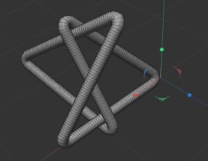
Then, we resized the spline to 6-7 cm for each dimension, and swept a circle of radius 0.3 cm around the spline, creating a tube around the knot. We did this to make the knots 3-dimensional, because we cannot 3D-print a spline (a 1-dimensional object in 3D space). To round the corners, we used the Chamfer function. Finally, we exported the models as .stl files and 3D printed them. In total, we designed all of the equilateral stick knots with three, four, five, six, and seven crossings. Additionally, we modeled knots with higher crossing number, such as 949, k11A1, and k12N603. The images above and below depict the 31 and 61 equilateral stick knot models.
Challenges and Observations:
- Scaling
- Self-intersections
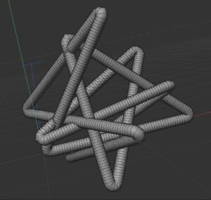
Initially, we did not scale our models to the appropriate size (suggested 6-7cm, or palm size). We also moved vertices around in the original 63 model, so the sticks lengths were altered, and we had to redo it. Additionally, the radius of the sticks was too small to neatly 3D print a label on the physical knot, so we decided to tape the labels on after the knots were printed. One interesting observation we made was increasing the radius of the tubes created self-intersections between the “tubes” that were not evident in the spline. The images above and below highlight self-intersections in the 61 and K12n630 models.


